Historically, the El Niño-Southern Oscillation (ENSO) cycle has been a major factor in a commodity trader's toolbox in understanding future productions/yields of agricultural commodities. The significance of the ENSO cycle on commodities can rise to astronomical levels, causing severe droughts or flooding in the Americas and Asia-Pacific regions.
Weather stations typically release ENSO forecasts that aim to explain general developments of El-Nino/La-Nina. In an ideal setting, these forecasts would be an accurate indicator of the likelihood of an El-Nino/La-Nina, which will be invaluable information to farmers, governments and commodity traders. In this project, we aim to explore the accuracy of historical ENSO forecasts and its performance.
We want to investigate two types of forecast data that is available:
raw ENSO SST forecast data is retrieved here: https://iri.columbia.edu/~forecast/ensofcst/Data/enso_plumes.json
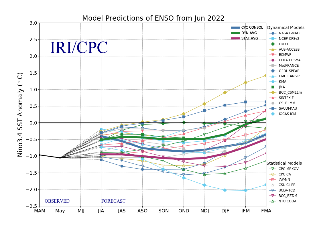
The ENSO predictions plume dataset contains the forecasted SST anomalies from various statistical and dynamical models from a range of third-party international forecasters. They range from weather agencies, government bodies to universities. Forecasted values start from Jan 2004 up until present. The dataset is compiled by the IRI from Columbia Climate School.
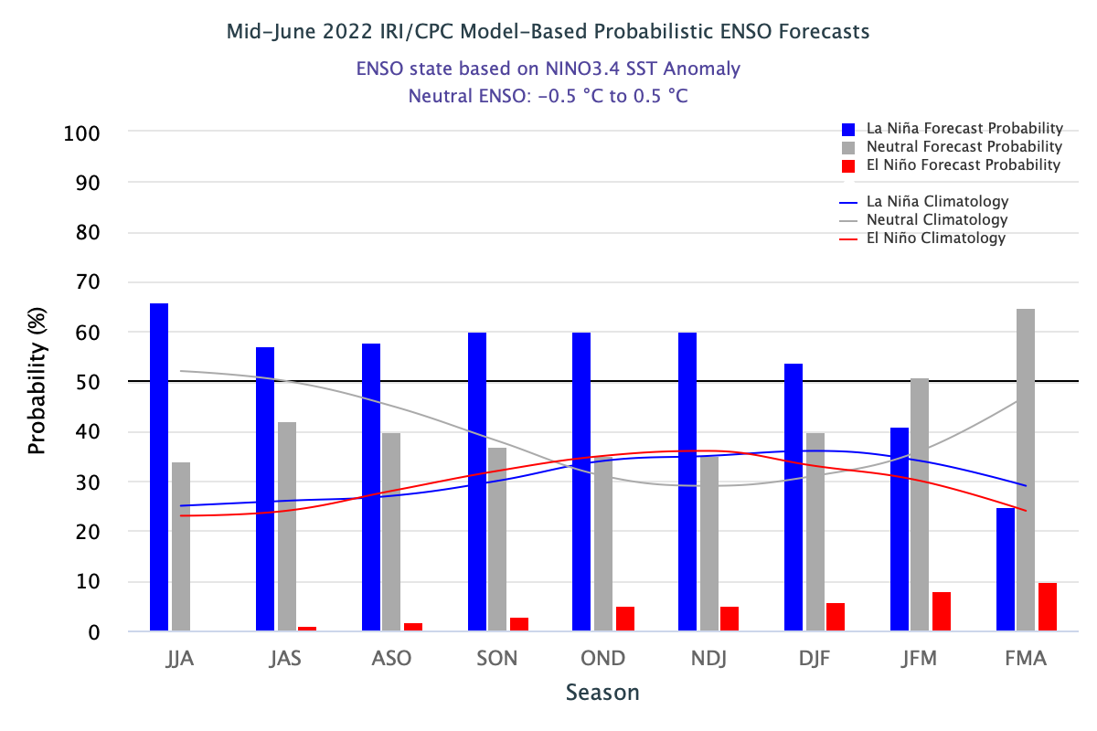
These models will provide monthly forecasts for up to nine overlapping 3-month periods. The 3-month periods are abbreviated by the starting letter of the month. For example, the 3-month period of Jan-Feb-Mar will be referred to as JFM.
For the simplicity of our research, we will convert the interpretation of the 3 month period into corresponding stand-alone months. For instance, in our subsequent visualisations, forecasted values for the 3-month period of Jan-Feb-Mar will be tagged to March (the last month of the 3-month period). This will be further observed later when we discuss the results of our visualisations. This will make it easier for us to plot time values instead of having to deal with 3-month periods on the x-axis.
On the 19th of each month, the IRI will release the updated forecasted values for the given month on its website.
To investigate the accuracy of the forecasted values, we will aggregate all values and take the average from all models. We will extract and transform the data from enso_plumes.json, after which visualize the trends and accuracy of the forecasts.
Import Statements
import pandas as pd
import numpy as np
import matplotlib.pyplot as plt
import json
import datetime
import seaborn as sn
Read json file
with open('enso_plumes.json', 'r') as myfile:
data = myfile.read()
plumes_data = json.loads(data)
df = pd.read_json('enso_plumes.json')
df.head()
years | |
---|---|
0 | {'months': [{'models': [{'data': [0.84, 0.8200... |
1 | {'months': [{'models': [{'data': [0.85, 0.66, ... |
2 | {'months': [{'models': [{'data': [-0.71, -0.66... |
3 | {'months': [{'models': [{'data': [0.58, 0.2, -... |
4 | {'months': [{'models': [{'data': [-1.82, -1.78... |
unwrap json nested data
# obtains all available years in the dataset and stores it into a pandas series
df = pd.json_normalize(plumes_data['years'])['year']
df
0 2004 1 2005 2 2006 3 2007 4 2008 5 2009 6 2010 7 2011 8 2012 9 2013 10 2014 11 2015 12 2016 13 2017 14 2018 15 2019 16 2020 17 2021 18 2022 Name: year, dtype: int64
def find_last_year(plumes_data):
'''
Takes in raw json forecast data, outputs an integer for slicing purposes
'''
helper = pd.json_normalize(plumes_data['years'])
entries_count = pd.json_normalize(helper['months']).count().sum()
return -(entries_count % 12)
# create a series of years according to data size
year_series = pd.concat([df]*12).sort_values()[:find_last_year(plumes_data)].reset_index().drop(columns='index')
year_series
year | |
---|---|
0 | 2004 |
1 | 2004 |
2 | 2004 |
3 | 2004 |
4 | 2004 |
... | ... |
217 | 2022 |
218 | 2022 |
219 | 2022 |
220 | 2022 |
221 | 2022 |
222 rows × 1 columns
df = pd.json_normalize(plumes_data, record_path = ['years', 'months'])
df['Year'] = year_series
df
models | month | observed | Year | |
---|---|---|---|---|
0 | [{'data': [0.84, 0.82, 0.87, 1.03, 1.17, 1.27,... | 0 | [{'data': 0.52, 'month': 'OND'}, {'data': 0.42... | 2004 |
1 | [{'data': [0.5, 0.56, 0.73, 1, 1.19, 1.28, 1.3... | 1 | [{'data': 0.39, 'month': 'NDJ'}, {'data': 0.22... | 2004 |
2 | [{'data': [0.33, 0.3, 0.28, 0.25, 0.21, 0.19, ... | 2 | [{'data': 0.27, 'month': 'DJF'}, {'data': 0.16... | 2004 |
3 | [{'data': [0.85, 1.11, 1.31, 1.35, 1.39, 1.49,... | 3 | [{'data': 0.1, 'month': 'JFM'}, {'data': 0, 'm... | 2004 |
4 | [{'data': [0.33, 0.38, 0.39, 0.4, 0.45, 0.55, ... | 4 | [{'data': 0, 'month': 'FMA'}, {'data': 0.1, 'm... | 2004 |
... | ... | ... | ... | ... |
217 | [{'model': 'NASA GMAO', 'type': 'Dynamical', '... | 1 | [{'month': 'NDJ', 'data': -0.94}, {'month': 'J... | 2022 |
218 | [{'model': 'NASA GMAO', 'type': 'Dynamical', '... | 2 | [{'month': 'DJF', 'data': -0.8633333333333333}... | 2022 |
219 | [{'model': 'NCEP CFSv2', 'type': 'Dynamical', ... | 3 | [{'month': 'JFM', 'data': -0.81}, {'month': 'M... | 2022 |
220 | [{'model': 'NASA GMAO', 'type': 'Dynamical', '... | 4 | [{'month': 'FMA', 'data': -0.85}, {'month': 'A... | 2022 |
221 | [{'model': 'NASA GMAO', 'type': 'Dynamical', '... | 5 | [{'month': 'MAM', 'data': -0.9633333333333333}... | 2022 |
222 rows × 4 columns
Calculating the average forecast value from all models
DATA_LENGTH = 9
def find_data_average(dict_lst):
'''
input: list of dictionaries with data, or series with dictionaries
output: list of average forecast data for each 3 month period, length 9
'''
final_lst = []
#filter out None values in dict_lst
dict_lst = list(filter(None, dict_lst))
for index in range(DATA_LENGTH):
value_lst = []
for dict in dict_lst:
try:
# try to catch error if there are Nan values, continue with the loop if there is
# if no Nan values, check if data is == -999 (which means data is not available)
# else, append value to value_lst
dict['data'][index] == -999
except:
continue
else:
if dict['data'][index] == -999:
continue
else:
value_lst.append(dict['data'][index])
average = sum(value_lst) / len(value_lst)
final_lst.append(average)
return final_lst
Create average forecast list for each time period
model_df = pd.json_normalize(df['models'])
avg_forecast_lst = []
for index, row in model_df.iterrows():
avg_forecast_lst.append(find_data_average(row))
df['Average_Forecast'] = avg_forecast_lst
df
models | month | observed | Year | Average_Forecast | |
---|---|---|---|---|---|
0 | [{'data': [0.84, 0.82, 0.87, 1.03, 1.17, 1.27,... | 0 | [{'data': 0.52, 'month': 'OND'}, {'data': 0.42... | 2004 | [0.37736842105263163, 0.3647368421052632, 0.36... |
1 | [{'data': [0.5, 0.56, 0.73, 1, 1.19, 1.28, 1.3... | 1 | [{'data': 0.39, 'month': 'NDJ'}, {'data': 0.22... | 2004 | [0.318421052631579, 0.33894736842105266, 0.377... |
2 | [{'data': [0.33, 0.3, 0.28, 0.25, 0.21, 0.19, ... | 2 | [{'data': 0.27, 'month': 'DJF'}, {'data': 0.16... | 2004 | [0.22526315789473692, 0.23894736842105263, 0.2... |
3 | [{'data': [0.85, 1.11, 1.31, 1.35, 1.39, 1.49,... | 3 | [{'data': 0.1, 'month': 'JFM'}, {'data': 0, 'm... | 2004 | [0.18736842105263163, 0.26789473684210524, 0.3... |
4 | [{'data': [0.33, 0.38, 0.39, 0.4, 0.45, 0.55, ... | 4 | [{'data': 0, 'month': 'FMA'}, {'data': 0.1, 'm... | 2004 | [0.14947368421052634, 0.22684210526315793, 0.2... |
... | ... | ... | ... | ... | ... |
217 | [{'model': 'NASA GMAO', 'type': 'Dynamical', '... | 1 | [{'month': 'NDJ', 'data': -0.94}, {'month': 'J... | 2022 | [-0.701537666781178, -0.5952292634642763, -0.4... |
218 | [{'model': 'NASA GMAO', 'type': 'Dynamical', '... | 2 | [{'month': 'DJF', 'data': -0.8633333333333333}... | 2022 | [-0.7272832916666667, -0.6016736666666666, -0.... |
219 | [{'model': 'NCEP CFSv2', 'type': 'Dynamical', ... | 3 | [{'month': 'JFM', 'data': -0.81}, {'month': 'M... | 2022 | [-0.6968667326689882, -0.5918087164555783, -0.... |
220 | [{'model': 'NASA GMAO', 'type': 'Dynamical', '... | 4 | [{'month': 'FMA', 'data': -0.85}, {'month': 'A... | 2022 | [-0.7512772944680615, -0.6362945096233904, -0.... |
221 | [{'model': 'NASA GMAO', 'type': 'Dynamical', '... | 5 | [{'month': 'MAM', 'data': -0.9633333333333333}... | 2022 | [-0.6317026030104692, -0.5803548643897951, -0.... |
222 rows × 5 columns
Further normalizing of json data
observed_df = pd.json_normalize(df['observed'])
observed_df
0 | 1 | |
---|---|---|
0 | {'data': 0.52, 'month': 'OND'} | {'data': 0.42, 'month': 'Dec'} |
1 | {'data': 0.39, 'month': 'NDJ'} | {'data': 0.22, 'month': 'Jan'} |
2 | {'data': 0.27, 'month': 'DJF'} | {'data': 0.16, 'month': 'Feb'} |
3 | {'data': 0.1, 'month': 'JFM'} | {'data': 0, 'month': 'Mar'} |
4 | {'data': 0, 'month': 'FMA'} | {'data': 0.1, 'month': 'Apr'} |
... | ... | ... |
217 | {'month': 'NDJ', 'data': -0.94} | {'month': 'Jan', 'data': -0.92} |
218 | {'month': 'DJF', 'data': -0.8633333333333333} | {'month': 'Feb', 'data': -0.71} |
219 | {'month': 'JFM', 'data': -0.81} | {'month': 'Mar', 'data': -0.89} |
220 | {'month': 'FMA', 'data': -0.85} | {'month': 'Apr', 'data': -0.95} |
221 | {'month': 'MAM', 'data': -0.9633333333333333} | {'month': 'May', 'data': -1.05} |
222 rows × 2 columns
# create dataframe of observed SST anomaly values for 3 month average period
mths3_df = pd.json_normalize(observed_df[0]).rename(columns = {
'data': 'Observed_3MTH', 'month': '3MTH'
})
# create dataframe of observed SST anomaly values for 1 month period
mths_df = pd.json_normalize(observed_df[1]).rename(columns = {
'data': 'Observed_Month', 'month': 'Month'
})
# merge both dataframes together
new_observed_df = pd.concat([mths3_df, mths_df], axis = 1)
# merge with original df
df = pd.concat([df, new_observed_df], axis = 1)
df.head()
models | month | observed | Year | Average_Forecast | Observed_3MTH | 3MTH | Observed_Month | Month | |
---|---|---|---|---|---|---|---|---|---|
0 | [{'data': [0.84, 0.82, 0.87, 1.03, 1.17, 1.27,... | 0 | [{'data': 0.52, 'month': 'OND'}, {'data': 0.42... | 2004 | [0.37736842105263163, 0.3647368421052632, 0.36... | 0.52 | OND | 0.42 | Dec |
1 | [{'data': [0.5, 0.56, 0.73, 1, 1.19, 1.28, 1.3... | 1 | [{'data': 0.39, 'month': 'NDJ'}, {'data': 0.22... | 2004 | [0.318421052631579, 0.33894736842105266, 0.377... | 0.39 | NDJ | 0.22 | Jan |
2 | [{'data': [0.33, 0.3, 0.28, 0.25, 0.21, 0.19, ... | 2 | [{'data': 0.27, 'month': 'DJF'}, {'data': 0.16... | 2004 | [0.22526315789473692, 0.23894736842105263, 0.2... | 0.27 | DJF | 0.16 | Feb |
3 | [{'data': [0.85, 1.11, 1.31, 1.35, 1.39, 1.49,... | 3 | [{'data': 0.1, 'month': 'JFM'}, {'data': 0, 'm... | 2004 | [0.18736842105263163, 0.26789473684210524, 0.3... | 0.10 | JFM | 0.00 | Mar |
4 | [{'data': [0.33, 0.38, 0.39, 0.4, 0.45, 0.55, ... | 4 | [{'data': 0, 'month': 'FMA'}, {'data': 0.1, 'm... | 2004 | [0.14947368421052634, 0.22684210526315793, 0.2... | 0.00 | FMA | 0.10 | Apr |
# drop observed column
df = df.drop(columns = 'observed')
df.head()
models | month | Year | Average_Forecast | Observed_3MTH | 3MTH | Observed_Month | Month | |
---|---|---|---|---|---|---|---|---|
0 | [{'data': [0.84, 0.82, 0.87, 1.03, 1.17, 1.27,... | 0 | 2004 | [0.37736842105263163, 0.3647368421052632, 0.36... | 0.52 | OND | 0.42 | Dec |
1 | [{'data': [0.5, 0.56, 0.73, 1, 1.19, 1.28, 1.3... | 1 | 2004 | [0.318421052631579, 0.33894736842105266, 0.377... | 0.39 | NDJ | 0.22 | Jan |
2 | [{'data': [0.33, 0.3, 0.28, 0.25, 0.21, 0.19, ... | 2 | 2004 | [0.22526315789473692, 0.23894736842105263, 0.2... | 0.27 | DJF | 0.16 | Feb |
3 | [{'data': [0.85, 1.11, 1.31, 1.35, 1.39, 1.49,... | 3 | 2004 | [0.18736842105263163, 0.26789473684210524, 0.3... | 0.10 | JFM | 0.00 | Mar |
4 | [{'data': [0.33, 0.38, 0.39, 0.4, 0.45, 0.55, ... | 4 | 2004 | [0.14947368421052634, 0.22684210526315793, 0.2... | 0.00 | FMA | 0.10 | Apr |
# add 1 to month value to more intuitive understanding (1 -> Jan, 2 -> Feb etc.)
df['month'] = df['month'] + 1
# create datetime column
df['Date'] = pd.to_datetime(df[['Year', 'month']].assign(DAY=1))
df.head()
models | month | Year | Average_Forecast | Observed_3MTH | 3MTH | Observed_Month | Month | Date | |
---|---|---|---|---|---|---|---|---|---|
0 | [{'data': [0.84, 0.82, 0.87, 1.03, 1.17, 1.27,... | 1 | 2004 | [0.37736842105263163, 0.3647368421052632, 0.36... | 0.52 | OND | 0.42 | Dec | 2004-01-01 |
1 | [{'data': [0.5, 0.56, 0.73, 1, 1.19, 1.28, 1.3... | 2 | 2004 | [0.318421052631579, 0.33894736842105266, 0.377... | 0.39 | NDJ | 0.22 | Jan | 2004-02-01 |
2 | [{'data': [0.33, 0.3, 0.28, 0.25, 0.21, 0.19, ... | 3 | 2004 | [0.22526315789473692, 0.23894736842105263, 0.2... | 0.27 | DJF | 0.16 | Feb | 2004-03-01 |
3 | [{'data': [0.85, 1.11, 1.31, 1.35, 1.39, 1.49,... | 4 | 2004 | [0.18736842105263163, 0.26789473684210524, 0.3... | 0.10 | JFM | 0.00 | Mar | 2004-04-01 |
4 | [{'data': [0.33, 0.38, 0.39, 0.4, 0.45, 0.55, ... | 5 | 2004 | [0.14947368421052634, 0.22684210526315793, 0.2... | 0.00 | FMA | 0.10 | Apr | 2004-05-01 |
from datetime import datetime
from dateutil.relativedelta import relativedelta
def get_forecast_mth(date):
'''
Takes in the date of data release, returns the equivalent 3 month rolling month
Example: Jan 2022 -> Mar 2022 (JFM)
'''
delta = relativedelta(months = 2)
return date + delta
def get_observed_mth(date):
'''
Takes in the date of data release, returns the date of latest observed data released
Observed data is always released with a 1 month lag
'''
delta = relativedelta(months = 1)
return date - delta
def create_date_df(date, forecast_list):
'''
create a df of dates corresponding to a set of SST anomaly forecasts
'''
lst = [date.replace(day=1)]
for i in range(len(forecast_list) - 1):
lst.append((lst[-1] + relativedelta(months = 1)).replace(day=1))
return pd.DataFrame(lst)
def create_forecast_df(forecast_list, date):
'''
create a dataframe of forecasts and dates at each specific time period
'''
data_df = pd.DataFrame(forecast_list)
data_df.columns = ['Forecast']
first_date = get_forecast_mth(date)
date_df = create_date_df(first_date, forecast_list)
date_df.columns = ['Date']
forecast_df = pd.concat([data_df, date_df], axis = 1)
forecast_df.set_index('Date', inplace = True)
return forecast_df
#from df, create a dictionary that stores all the different forecast values according to the starting month
#key = date, values = dataframe of forecasted values with forecasted month
forecast_dict = {date:create_forecast_df(forecast, date) for forecast, date in zip(df['Average_Forecast'], df['Date'])}
forecast_dict[datetime(2004,1,1)]
Forecast | |
---|---|
Date | |
2004-03-01 | 0.377368 |
2004-04-01 | 0.364737 |
2004-05-01 | 0.365000 |
2004-06-01 | 0.388824 |
2004-07-01 | 0.412941 |
2004-08-01 | 0.389375 |
2004-09-01 | 0.402667 |
2004-10-01 | 0.350000 |
2004-11-01 | 0.331667 |
observed_df = df[['Date', 'Observed_3MTH']]
observed_df['Date'] = observed_df['Date'].apply(lambda x: get_observed_mth(x))
observed_df.set_index('Date', inplace = True)
observed_df
C:\Users\raych\AppData\Local\Temp\ipykernel_20036\3176640886.py:2: SettingWithCopyWarning: A value is trying to be set on a copy of a slice from a DataFrame. Try using .loc[row_indexer,col_indexer] = value instead See the caveats in the documentation: https://pandas.pydata.org/pandas-docs/stable/user_guide/indexing.html#returning-a-view-versus-a-copy observed_df['Date'] = observed_df['Date'].apply(lambda x: get_observed_mth(x))
Observed_3MTH | |
---|---|
Date | |
2003-12-01 | 0.520000 |
2004-01-01 | 0.390000 |
2004-02-01 | 0.270000 |
2004-03-01 | 0.100000 |
2004-04-01 | 0.000000 |
... | ... |
2022-01-01 | -0.940000 |
2022-02-01 | -0.863333 |
2022-03-01 | -0.810000 |
2022-04-01 | -0.850000 |
2022-05-01 | -0.963333 |
222 rows × 1 columns
# double check for any null values
observed_df.isnull().any()
Observed_3MTH False dtype: bool
Using Matplotlib
import matplotlib.ticker as ticker
import matplotlib.dates as mdates
#Matplotlib Plotting
fig = plt.figure(figsize=[20,10])
ax = fig.add_subplot(1,1,1)
plt.grid()
plt.title('ENSO Forecast and Actual Values')
plt.axhline(y = 0.5, color = 'r', linestyle = 'dashed')
plt.axhline(y = -0.5, color = 'b', linestyle = 'dashed')
plt.ylabel('SST Anomaly Degree C')
for key, df in forecast_dict.items():
plt.plot(df.index, df['Forecast'])
plt.plot(observed_df.index, observed_df['Observed_3MTH'], 'k')
ax.xaxis.set_major_locator(mdates.YearLocator(1))
plt.show()
Using Plotly
import plotly
import plotly.offline as pyo
import plotly.graph_objects as go
from plotly.subplots import make_subplots
import plotly.express as px
pyo.init_notebook_mode(connected=True)
#print(data_return.info())
pd.options.plotting.backend = 'plotly'
# Creating custom color list to label different months (each month will have a distinct color)
color_discrete_sequence=px.colors.qualitative.Plotly + ["#bcbd22", "#316395"]
custom_color = ["#e60049", "#0bb4ff", "#50e991", "#e6d800", "#9b19f5", "#ffa300", "#dc0ab4", "#b3d4ff", "#00bfa0", "#a52a2a", "#483d8b", "#8b0000"]
print(color_discrete_sequence)
['#636EFA', '#EF553B', '#00CC96', '#AB63FA', '#FFA15A', '#19D3F3', '#FF6692', '#B6E880', '#FF97FF', '#FECB52', '#bcbd22', '#316395']
def get_color(seq,i):
'''
function for plotly color assigning
seq = dictionary, i = int
'''
return seq[i%len(seq)]
# Using plotly graph objects
fig = go.Figure(layout=go.Layout(height = 750, width = 1500))
i = 0
# iterate over forecast_dict to plot forecast lines
for key, df in forecast_dict.items():
fig.add_trace(go.Scatter(x = df.index, y = df['Forecast'], name = key.strftime('%Y-%m-%d'), marker = {'color': get_color(color_discrete_sequence, i)}))
i += 1
# add observed sst line
fig.add_trace(go.Scatter(x = observed_df.index, y = observed_df['Observed_3MTH'], mode = 'lines+markers', name = 'Observed', line = dict(color = 'black')))
# add elnino sst threshold
fig.add_hline(y=0.5, line_color = 'red', line_dash = 'dash')
# add lanina sst threshold
fig.add_hline(y = -0.5, line_color = 'blue', line_dash = 'dash')
fig.update_yaxes(title_text="SST Anomalies (℃)")
fig.update_xaxes(dtick="M12", tickformat="%Y", hoverformat = "%B %Y")
fig.update_layout(title = 'ENSO Forecast and Observed Values')
fig.show()
Next, we wanted to visualise the ENSO forecasts values grouped by forecast horizon.
Forecasts will be grouped according to their forecast horizon (T+1, T+2, T+3 ...)
# Forecast range limit is 9, which means T+9 will be the furthest forecast horizon provided by the forecasting models
FORECAST_RANGE = 9
master_df = pd.DataFrame()
# loop over FORECAST_RANGE
for i in range(FORECAST_RANGE):
t_df = pd.DataFrame()
# loop over all forecasts in forecast_dict
for key, df in forecast_dict.items():
# retrive only the ith forecast horizon
t_df = pd.concat([t_df, df.iloc[i]], axis = 1, join = 'outer')
#transpose in order to get forecast horizon as a column
t_df = t_df.transpose()
#rename the forecast horizon to the corresponding period
t_df.rename(columns = {'Forecast': 'T+'+str(i+1)}, inplace = True)
master_df = pd.concat([master_df, t_df], axis = 1, join = 'outer')
master_df
T+1 | T+2 | T+3 | T+4 | T+5 | T+6 | T+7 | T+8 | T+9 | |
---|---|---|---|---|---|---|---|---|---|
2004-03-01 | 0.377368 | NaN | NaN | NaN | NaN | NaN | NaN | NaN | NaN |
2004-04-01 | 0.318421 | 0.364737 | NaN | NaN | NaN | NaN | NaN | NaN | NaN |
2004-05-01 | 0.225263 | 0.338947 | 0.365000 | NaN | NaN | NaN | NaN | NaN | NaN |
2004-06-01 | 0.187368 | 0.238947 | 0.377222 | 0.388824 | NaN | NaN | NaN | NaN | NaN |
2004-07-01 | 0.149474 | 0.267895 | 0.268889 | 0.439412 | 0.412941 | NaN | NaN | NaN | NaN |
... | ... | ... | ... | ... | ... | ... | ... | ... | ... |
2022-12-01 | NaN | NaN | NaN | NaN | -0.691075 | -0.717113 | -0.590189 | -0.113169 | 0.109567 |
2023-01-01 | NaN | NaN | NaN | NaN | NaN | -0.697723 | -0.681231 | -0.435382 | -0.070961 |
2023-02-01 | NaN | NaN | NaN | NaN | NaN | NaN | -0.581102 | -0.438628 | -0.343234 |
2023-03-01 | NaN | NaN | NaN | NaN | NaN | NaN | NaN | -0.377385 | -0.274230 |
2023-04-01 | NaN | NaN | NaN | NaN | NaN | NaN | NaN | NaN | -0.173767 |
230 rows × 9 columns
observed_df
Observed_3MTH | |
---|---|
Date | |
2003-12-01 | 0.520000 |
2004-01-01 | 0.390000 |
2004-02-01 | 0.270000 |
2004-03-01 | 0.100000 |
2004-04-01 | 0.000000 |
... | ... |
2022-01-01 | -0.940000 |
2022-02-01 | -0.863333 |
2022-03-01 | -0.810000 |
2022-04-01 | -0.850000 |
2022-05-01 | -0.963333 |
222 rows × 1 columns
# add observed values into master_df
master_df = pd.concat([master_df,observed_df], axis = 1, join = 'outer')
master_df.index.name = 'Date'
master_df
T+1 | T+2 | T+3 | T+4 | T+5 | T+6 | T+7 | T+8 | T+9 | Observed_3MTH | |
---|---|---|---|---|---|---|---|---|---|---|
Date | ||||||||||
2003-12-01 | NaN | NaN | NaN | NaN | NaN | NaN | NaN | NaN | NaN | 0.52 |
2004-01-01 | NaN | NaN | NaN | NaN | NaN | NaN | NaN | NaN | NaN | 0.39 |
2004-02-01 | NaN | NaN | NaN | NaN | NaN | NaN | NaN | NaN | NaN | 0.27 |
2004-03-01 | 0.377368 | NaN | NaN | NaN | NaN | NaN | NaN | NaN | NaN | 0.10 |
2004-04-01 | 0.318421 | 0.364737 | NaN | NaN | NaN | NaN | NaN | NaN | NaN | 0.00 |
... | ... | ... | ... | ... | ... | ... | ... | ... | ... | ... |
2022-12-01 | NaN | NaN | NaN | NaN | -0.691075 | -0.717113 | -0.590189 | -0.113169 | 0.109567 | NaN |
2023-01-01 | NaN | NaN | NaN | NaN | NaN | -0.697723 | -0.681231 | -0.435382 | -0.070961 | NaN |
2023-02-01 | NaN | NaN | NaN | NaN | NaN | NaN | -0.581102 | -0.438628 | -0.343234 | NaN |
2023-03-01 | NaN | NaN | NaN | NaN | NaN | NaN | NaN | -0.377385 | -0.274230 | NaN |
2023-04-01 | NaN | NaN | NaN | NaN | NaN | NaN | NaN | NaN | -0.173767 | NaN |
233 rows × 10 columns
Correlation Matrix
master_df.corr()
T+1 | T+2 | T+3 | T+4 | T+5 | T+6 | T+7 | T+8 | T+9 | Observed_3MTH | |
---|---|---|---|---|---|---|---|---|---|---|
T+1 | 1.000000 | 0.986440 | 0.956061 | 0.912314 | 0.853098 | 0.777716 | 0.702151 | 0.608637 | 0.521723 | 0.962568 |
T+2 | 0.986440 | 1.000000 | 0.984113 | 0.948502 | 0.895434 | 0.819630 | 0.743212 | 0.641022 | 0.547180 | 0.931677 |
T+3 | 0.956061 | 0.984113 | 1.000000 | 0.981264 | 0.938921 | 0.871505 | 0.794044 | 0.693413 | 0.591455 | 0.893632 |
T+4 | 0.912314 | 0.948502 | 0.981264 | 1.000000 | 0.976549 | 0.922497 | 0.852554 | 0.751193 | 0.653525 | 0.847277 |
T+5 | 0.853098 | 0.895434 | 0.938921 | 0.976549 | 1.000000 | 0.968081 | 0.909727 | 0.818709 | 0.719646 | 0.793296 |
T+6 | 0.777716 | 0.819630 | 0.871505 | 0.922497 | 0.968081 | 1.000000 | 0.964124 | 0.890103 | 0.804195 | 0.725356 |
T+7 | 0.702151 | 0.743212 | 0.794044 | 0.852554 | 0.909727 | 0.964124 | 1.000000 | 0.948082 | 0.872898 | 0.663910 |
T+8 | 0.608637 | 0.641022 | 0.693413 | 0.751193 | 0.818709 | 0.890103 | 0.948082 | 1.000000 | 0.944885 | 0.578199 |
T+9 | 0.521723 | 0.547180 | 0.591455 | 0.653525 | 0.719646 | 0.804195 | 0.872898 | 0.944885 | 1.000000 | 0.488574 |
Observed_3MTH | 0.962568 | 0.931677 | 0.893632 | 0.847277 | 0.793296 | 0.725356 | 0.663910 | 0.578199 | 0.488574 | 1.000000 |
sn.heatmap(master_df.corr(), annot=True)
plt.show()
Looking at the correlation matrix, forecasted values with near horizon have very high correlations when compared to the observed values, which is intuitive as strength of forecasted values would be stronger for short term horizons. The strength of the forecasts decreases as it attempts to predict values further into the future.
# Using plotly graph objects
fig1_2 = go.Figure(layout=go.Layout(height = 750, width = 1500))
i = 0
for col in master_df.columns[:-1]:
fig1_2.add_trace(go.Line(x = master_df.index, y = master_df[col], name = col, marker = {'color': get_color(color_discrete_sequence, i)}))
i += 1
fig1_2.add_trace(go.Line(x = observed_df.index, y = observed_df['Observed_3MTH'], mode = 'lines+markers', name = 'Observed', line = dict(color = 'black')))
fig1_2.add_hline(y=0.5, line_color = 'red', line_dash = 'dash')
fig1_2.add_hline(y = -0.5, line_color = 'blue', line_dash = 'dash')
fig1_2.update_yaxes(title_text="SST Anomalies (℃)")
fig1_2.update_xaxes(dtick="M12", tickformat="%Y", hoverformat = "%B %Y")
fig1_2.update_layout(title = 'ENSO Forecasts grouped by forecast horizon')
fig1_2.show()
c:\Users\raych\AppData\Local\Programs\Python\Python39\lib\site-packages\plotly\graph_objs\_deprecations.py:378: DeprecationWarning: plotly.graph_objs.Line is deprecated. Please replace it with one of the following more specific types - plotly.graph_objs.scatter.Line - plotly.graph_objs.layout.shape.Line - etc.
The T+1 forecast horizon tracks the observed values the best. As the forecast horizon increases, the predictions start to become less precise.
We will define the calculation of errors as: observed values - predicted values
#errors = observed - predicted
errors_df = pd.DataFrame()
for col in master_df.columns[:-1]:
errors_df[col] = master_df['Observed_3MTH'].apply(lambda x: np.abs(x)) - master_df[col].apply(lambda x: np.abs(x))
errors_df['Observed_3MTH'] = master_df['Observed_3MTH']
errors_df
T+1 | T+2 | T+3 | T+4 | T+5 | T+6 | T+7 | T+8 | T+9 | Observed_3MTH | |
---|---|---|---|---|---|---|---|---|---|---|
Date | ||||||||||
2003-12-01 | NaN | NaN | NaN | NaN | NaN | NaN | NaN | NaN | NaN | 0.52 |
2004-01-01 | NaN | NaN | NaN | NaN | NaN | NaN | NaN | NaN | NaN | 0.39 |
2004-02-01 | NaN | NaN | NaN | NaN | NaN | NaN | NaN | NaN | NaN | 0.27 |
2004-03-01 | -0.277368 | NaN | NaN | NaN | NaN | NaN | NaN | NaN | NaN | 0.10 |
2004-04-01 | -0.318421 | -0.364737 | NaN | NaN | NaN | NaN | NaN | NaN | NaN | 0.00 |
... | ... | ... | ... | ... | ... | ... | ... | ... | ... | ... |
2022-12-01 | NaN | NaN | NaN | NaN | NaN | NaN | NaN | NaN | NaN | NaN |
2023-01-01 | NaN | NaN | NaN | NaN | NaN | NaN | NaN | NaN | NaN | NaN |
2023-02-01 | NaN | NaN | NaN | NaN | NaN | NaN | NaN | NaN | NaN | NaN |
2023-03-01 | NaN | NaN | NaN | NaN | NaN | NaN | NaN | NaN | NaN | NaN |
2023-04-01 | NaN | NaN | NaN | NaN | NaN | NaN | NaN | NaN | NaN | NaN |
233 rows × 10 columns
Finding the absolute mean error for each forecast horizon
errors_df.apply(lambda x: np.abs(x)).mean()
T+1 0.169763 T+2 0.224518 T+3 0.270483 T+4 0.315303 T+5 0.358647 T+6 0.394159 T+7 0.420820 T+8 0.440998 T+9 0.452018 Observed_3MTH 0.636802 dtype: float64
Forecast horizon T+1 has the lowest absolute mean error of 0.16℃.
# Using plotly graph objects
fig1_3 = go.Figure(layout=go.Layout(height = 750, width = 1500))
i = 0
for col in errors_df.columns[:-1]:
fig1_3.add_trace(go.Scatter(x = errors_df.index, y = errors_df[col], name = col, marker = {'color': get_color(color_discrete_sequence, i)}))
i += 1
fig1_3.add_trace(go.Scatter(x = observed_df.index, y = observed_df['Observed_3MTH'], mode = 'lines+markers', name = 'Observed', line = dict(color = 'black')))
fig1_3.add_hline(y=0.5, line_color = 'red', line_dash = 'dash')
fig1_3.add_hline(y = -0.5, line_color = 'blue', line_dash = 'dash')
fig1_3.update_yaxes(title_text="SST Anomalies (℃)")
fig1_3.update_xaxes(dtick="M12", tickformat="%Y", hoverformat = "%B %Y")
fig1_3.update_layout(title = 'ENSO Forecasts Errors')
fig1_3.show()
raw IRI probabilistic forecast data is retrieved here: https://iri.columbia.edu/~forecast/ensofcst/Data/enso_iri_prob.json
The IRI probabilistic ENSO forecast shows the likelihood of an El-Nino, La-Nina or a neutral state in terms of probability. These probability forecasts are calculated based on regression, with the inputs being the SST anomalies forecasts from the various models. The probabilities across the three states will sum up to 1.
Similar to the SST forecasts, the IRI probabilistic forecast provides monthly forecasts for up to nine 3-month overlapping periods. Probabilistic forecasts data starts from June 2003 up til present.
On the 19th of each month, the IRI will release the updated forecasted values for the given month on its website.
with open('enso_iri_prob.json', 'r') as myfile:
data = myfile.read()
enso_iri_data = json.loads(data)
# IRI probabilities started from June 2003, which means there are only 7 2003 monthly probabiltiies released
df = pd.json_normalize(enso_iri_data['years'])['year']
def find_last_year_iri(enso_iri_data):
helper = pd.json_normalize(enso_iri_data['years'])
# the addition of 5 is to make up for the fact that there are only 7 2003 monthly probabilities released (12 - 7 = 5)
entries_count = pd.json_normalize(helper['months']).count().sum() + 5
return -(entries_count % 12)
# crate year series
year_series = pd.concat([df]*12).sort_values()[5:find_last_year_iri(enso_iri_data)].reset_index().drop(columns='index')
year_series
year | |
---|---|
0 | 2003 |
1 | 2003 |
2 | 2003 |
3 | 2003 |
4 | 2003 |
... | ... |
224 | 2022 |
225 | 2022 |
226 | 2022 |
227 | 2022 |
228 | 2022 |
229 rows × 1 columns
df = pd.json_normalize(enso_iri_data, record_path = ['years', 'months'])
df['Year'] = year_series
df
month | probabilities | Year | |
---|---|---|---|
0 | 5 | [{'elnino': 0, 'lanina': 45, 'neutral': 55, 's... | 2003 |
1 | 6 | [{'elnino': 18, 'lanina': 30, 'neutral': 52, '... | 2003 |
2 | 7 | [{'elnino': 12, 'lanina': 12, 'neutral': 76, '... | 2003 |
3 | 8 | [{'elnino': 10, 'lanina': 10, 'neutral': 80, '... | 2003 |
4 | 9 | [{'elnino': 15, 'lanina': 5, 'neutral': 80, 's... | 2003 |
... | ... | ... | ... |
224 | 1 | [{'season': 'FMA', 'lanina': 79, 'neutral': 21... | 2022 |
225 | 2 | [{'season': 'MAM', 'lanina': 86, 'neutral': 14... | 2022 |
226 | 3 | [{'season': 'AMJ', 'lanina': 80, 'neutral': 20... | 2022 |
227 | 4 | [{'season': 'MJJ', 'lanina': 81, 'neutral': 19... | 2022 |
228 | 5 | [{'season': 'JJA', 'lanina': 66, 'neutral': 34... | 2022 |
229 rows × 3 columns
df['month'] = df['month'] + 1
# create datetime column, forecasts are released on the 19th of each month
df['Date'] = pd.to_datetime(df[['Year', 'month']].assign(DAY=19))
df.head()
month | probabilities | Year | Date | |
---|---|---|---|---|
0 | 6 | [{'elnino': 0, 'lanina': 45, 'neutral': 55, 's... | 2003 | 2003-06-19 |
1 | 7 | [{'elnino': 18, 'lanina': 30, 'neutral': 52, '... | 2003 | 2003-07-19 |
2 | 8 | [{'elnino': 12, 'lanina': 12, 'neutral': 76, '... | 2003 | 2003-08-19 |
3 | 9 | [{'elnino': 10, 'lanina': 10, 'neutral': 80, '... | 2003 | 2003-09-19 |
4 | 10 | [{'elnino': 15, 'lanina': 5, 'neutral': 80, 's... | 2003 | 2003-10-19 |
df.probabilities[0]
[{'elnino': 0, 'lanina': 45, 'neutral': 55, 'season': 'JJA'}, {'elnino': 1, 'lanina': 45, 'neutral': 54, 'season': 'JAS'}, {'elnino': 1, 'lanina': 45, 'neutral': 54, 'season': 'ASO'}, {'elnino': 1, 'lanina': 45, 'neutral': 54, 'season': 'SON'}, {'elnino': 1, 'lanina': 45, 'neutral': 54, 'season': 'OND'}, {'elnino': 2, 'lanina': 44, 'neutral': 54, 'season': 'NDJ'}, {'elnino': 5, 'lanina': 42, 'neutral': 53, 'season': 'DJF'}, {'elnino': 9, 'lanina': 40, 'neutral': 51, 'season': 'JFM'}, {'elnino': 13, 'lanina': 37, 'neutral': 50, 'season': 'FMA'}, {'elnino': 18, 'lanina': 32, 'neutral': 50, 'season': 'MAM'}]
def aggregate_prob(list_of_dict):
'''
function to transform the above list of dictionaries into a dictionary, with the key being the event, and value being the list of
forecasted values
'''
final_dict = {}
final_dict['elnino'] = []
final_dict['lanina'] = []
final_dict['neutral'] = []
final_dict['season'] = []
for i in list_of_dict:
for key,value in i.items():
final_dict[key].append(value)
return final_dict
df['probabilities'] = df['probabilities'].apply(lambda x: aggregate_prob(x))
df.head()
month | probabilities | Year | Date | |
---|---|---|---|---|
0 | 6 | {'elnino': [0, 1, 1, 1, 1, 2, 5, 9, 13, 18], '... | 2003 | 2003-06-19 |
1 | 7 | {'elnino': [18, 18, 18, 18, 18, 18, 19, 20, 22... | 2003 | 2003-07-19 |
2 | 8 | {'elnino': [12, 13, 14, 15, 17, 19, 21, 23, 25... | 2003 | 2003-08-19 |
3 | 9 | {'elnino': [10, 11, 12, 13, 15, 17, 19, 22, 24... | 2003 | 2003-09-19 |
4 | 10 | {'elnino': [15, 16, 17, 18, 20, 22, 24, 25, 25... | 2003 | 2003-10-19 |
from datetime import datetime
from dateutil.relativedelta import relativedelta
# Example of how one entry will appear in df.probabilities
pd.DataFrame(df.probabilities[0])
elnino | lanina | neutral | season | |
---|---|---|---|---|
0 | 0 | 45 | 55 | JJA |
1 | 1 | 45 | 54 | JAS |
2 | 1 | 45 | 54 | ASO |
3 | 1 | 45 | 54 | SON |
4 | 1 | 45 | 54 | OND |
5 | 2 | 44 | 54 | NDJ |
6 | 5 | 42 | 53 | DJF |
7 | 9 | 40 | 51 | JFM |
8 | 13 | 37 | 50 | FMA |
9 | 18 | 32 | 50 | MAM |
def create_probs_df(forecast_dict, date):
'''
Creates a dataframe of the probabilistic forecasts and the corresponding dates
'''
def get_forecast_mth(date):
'''
Takes in the date of data release, returns the equivalent 3 month rolling month
Example: Jan 2022 -> Mar 2022 (JFM)
'''
delta = relativedelta(months = 2)
return date + delta
def create_probs_date_df(date, forecast_dict):
'''
Creates a date df for IRI probabilistic forecasts
'''
lst = [date.replace(day=1)]
# iterate over the length of the forecast values
for i in range(len(next(iter(forecast_dict.values()))) - 1):
lst.append((lst[-1] + relativedelta(months = 1)).replace(day = 1))
return pd.DataFrame(lst)
data_df = pd.DataFrame(forecast_dict)
first_date = get_forecast_mth(date)
date_df = create_probs_date_df(first_date, forecast_dict)
date_df.columns = ['Date']
forecast_df = pd.concat([data_df, date_df], axis = 1)
forecast_df.set_index('Date', inplace = True)
return forecast_df
#from df, create a dictionary that stores all the different forecast values according to the starting month
#key = date, values = dataframe of forecasted values with forecasted month
probs_dict = {date:create_probs_df(prob, date) for prob, date in zip(df['probabilities'], df['Date'])}
probs_dict[datetime(2003,6,19)]
elnino | lanina | neutral | season | |
---|---|---|---|---|
Date | ||||
2003-08-01 | 0 | 45 | 55 | JJA |
2003-09-01 | 1 | 45 | 54 | JAS |
2003-10-01 | 1 | 45 | 54 | ASO |
2003-11-01 | 1 | 45 | 54 | SON |
2003-12-01 | 1 | 45 | 54 | OND |
2004-01-01 | 2 | 44 | 54 | NDJ |
2004-02-01 | 5 | 42 | 53 | DJF |
2004-03-01 | 9 | 40 | 51 | JFM |
2004-04-01 | 13 | 37 | 50 | FMA |
2004-05-01 | 18 | 32 | 50 | MAM |
import plotly
import plotly.offline as pyo
import plotly.graph_objects as go
from plotly.subplots import make_subplots
import plotly.express as px
pyo.init_notebook_mode(connected=True)
#print(data_return.info())
pd.options.plotting.backend = 'plotly'
fig1 = make_subplots(specs=[[{"secondary_y": True}]])
for key, df in probs_dict.items():
fig1.add_trace(go.Scatter(x = df.index, y = df['elnino'], mode = 'lines', name = key.strftime('%Y-%m-%d'), marker = {'color': 'red'}), secondary_y=False)
fig1.add_trace(go.Scatter(x = observed_df.index, y = observed_df['Observed_3MTH'], mode = 'lines+markers', name = 'Observed', line = dict(color = 'black')), secondary_y=True)
fig1.add_hline(y=0.5, line_color = 'red', line_dash = 'dash', secondary_y=True)
fig1.add_hline(y = -0.5, line_color = 'blue', line_dash = 'dash', secondary_y=True)
fig1.update_xaxes(dtick="M12", tickformat="%Y", hoverformat = "%B %Y")
fig1.update_yaxes(title_text="El Nino Probability (%)", secondary_y=False)
fig1.update_yaxes(title_text="Observed SST Anomalies (℃)", secondary_y=True)
fig1.update_layout(height = 750, width = 1500, title = 'El-Nino Probabilities')
fig1.show()
fig2 = make_subplots(specs=[[{"secondary_y": True}]])
for key, df in probs_dict.items():
fig2.add_trace(go.Scatter(x = df.index, y = df['lanina'], mode = 'lines', name = key.strftime('%Y-%m-%d'), marker = {'color': 'blue'}), secondary_y=False)
fig2.add_trace(go.Scatter(x = observed_df.index, y = observed_df['Observed_3MTH'], mode = 'lines+markers', name = 'Observed', line = dict(color = 'black')), secondary_y=True)
fig2.add_hline(y=0.5, line_color = 'red', line_dash = 'dash', secondary_y=True)
fig2.add_hline(y = -0.5, line_color = 'blue', line_dash = 'dash', secondary_y=True)
fig2.update_xaxes(dtick="M12", tickformat="%Y", hoverformat = "%B %Y")
fig2.update_yaxes(title_text="La Nina Probability (%)", secondary_y=False)
fig2.update_yaxes(title_text="Observed SST Anomalies (℃)", secondary_y=True)
fig2.update_layout(height = 750, width = 1500, title = 'La-Nina Probabilities')
fig2.show()
Transposing Data, to plot graphs according to T+1, T+2 etc.
Transposing El-Nino Data
FORECAST_RANGE = 9
t_1_list = []
elnino_df = pd.DataFrame()
for i in range(FORECAST_RANGE):
t_1_df = pd.DataFrame()
for key, df in probs_dict.items():
t_1_df = pd.concat([t_1_df, pd.DataFrame(df['elnino']).iloc[i]], axis = 1, join = 'outer')
t_1_df = t_1_df.transpose()
t_1_df.rename(columns = {'elnino': 'T+'+str(i+1)}, inplace = True)
elnino_df = pd.concat([elnino_df, t_1_df], axis = 1, join = 'outer')
Transposing La-Nina Data
FORECAST_RANGE = 9
t_1_list = []
lanina_df = pd.DataFrame()
for i in range(FORECAST_RANGE):
t_1_df = pd.DataFrame()
for key, df in probs_dict.items():
#print(df.iloc[i])
#print(len(df['elnino']))
t_1_df = pd.concat([t_1_df, pd.DataFrame(df['lanina']).iloc[i]], axis = 1, join = 'outer')
t_1_df = t_1_df.transpose()
t_1_df.rename(columns = {'lanina': 'T+'+str(i+1)}, inplace = True)
lanina_df = pd.concat([lanina_df, t_1_df], axis = 1, join = 'outer')
fig3 = make_subplots(specs=[[{"secondary_y": True}]])
for col in elnino_df.columns:
fig3.add_trace(go.Scatter(x = elnino_df.index, y = elnino_df[col], mode = 'lines+markers', name = col), secondary_y=False)
fig3.add_trace(go.Scatter(x = observed_df.index, y = observed_df['Observed_3MTH'], mode = 'lines+markers', name = 'Observed', line = dict(color = 'black')), secondary_y=True)
fig3.add_hline(y=0.5, line_color = 'red', line_dash = 'dash', secondary_y=True)
fig3.add_hline(y = -0.5, line_color = 'blue', line_dash = 'dash', secondary_y=True)
fig3.update_xaxes(dtick="M12", tickformat="%Y", hoverformat = "%B %Y")
fig3.update_yaxes(title_text="El Nino-La Nina Probability (%)", secondary_y=False)
fig3.update_yaxes(title_text="Observed SST Anomalies (℃)", secondary_y=True)
fig3.update_layout(height = 750, width = 1500, title = 'El-Nino Probabilities grouped by forecast horizon')
fig3.show()
After isolating the T+1 horizon and the observed SST Anomalies values, we can see that once the El-Nino probability hits 85% or above, an actual El-Nino (of various magnitudes) will surface. Sustained high probabilities after the initial forecast will strengthen the conviction of the occurence of an El-Nino.
fig4 = make_subplots(specs=[[{"secondary_y": True}]])
for col in lanina_df.columns:
fig4.add_trace(go.Scatter(x = lanina_df.index, y = lanina_df[col], mode = 'lines+markers', name = col), secondary_y=False)
fig4.add_trace(go.Scatter(x = observed_df.index, y = observed_df['Observed_3MTH'], mode = 'lines+markers', name = 'Observed', line = dict(color = 'black')), secondary_y=True)
fig4.add_hline(y=0.5, line_color = 'red', line_dash = 'dash', secondary_y=True)
fig4.add_hline(y = -0.5, line_color = 'blue', line_dash = 'dash', secondary_y=True)
fig4.update_xaxes(dtick="M12", tickformat="%Y", hoverformat = "%B %Y")
fig4.update_yaxes(title_text="El Nino-La Nina Probability (%)", secondary_y=False)
fig4.update_yaxes(title_text="Observed SST Anomalies (℃)", secondary_y=True)
fig4.update_layout(height = 750, width = 1500, title = 'La-Nina Probabilities grouped by forecast horizon')
fig4.show()
Turning to La-Nina, after isolating the T+1 forecast horizon, we see similar patterns to that of El-Nino. High probabilities of a La-Nina occurence (85%) would likely mean an actual occurence.
The chances of a false positive is rare, in fact every time T+1 probability hits above 85%, an actual La-Nina event is observed.
with open('ENSO_forecasts_visualisations.html', 'a') as f:
f.write(fig.to_html(full_html=False, include_plotlyjs='cdn'))
f.write(fig1_2.to_html(full_html=False, include_plotlyjs='cdn'))
f.write(fig1_3.to_html(full_html=False, include_plotlyjs='cdn'))
f.write(fig1.to_html(full_html=False, include_plotlyjs='cdn'))
f.write(fig2.to_html(full_html=False, include_plotlyjs='cdn'))
f.write(fig3.to_html(full_html=False, include_plotlyjs='cdn'))
f.write(fig4.to_html(full_html=False, include_plotlyjs='cdn'))
Conclusion and Further Steps:
From our analysis, we observe that the forecasted values do provide reasonable predictions on future SST anomalies and thus probabilities of El-Nino/La-Nina occurences.
Even though forecasts are released up to nine months into the future, the accuracy of said forecasts degrades over time due to increasing uncertainty. Perhaps the most useful forecasts horizons to commodity traders/government bodies would be T+1 up to T+3.
Further work will be to conduct statistical analysis to discover potential relationships between ENSO SST anomalies forecasts and various outputs such as production/yield/prices of differing commodities. El-Nino/La-Nina has varying impact on different types of commodities from different regions, thus this analysis will have to be conducted on a micro scale.
statsmodels
from statsmodels.tsa.seasonal import seasonal_decompose
errors_df['T+1'].dropna()
Date 2004-03-01 -0.277368 2004-04-01 -0.318421 2004-05-01 -0.125263 2004-06-01 0.012632 2004-07-01 0.150526 ... 2022-01-01 -0.074175 2022-02-01 -0.150188 2022-03-01 -0.148765 2022-04-01 0.148462 2022-05-01 0.236050 Freq: MS, Name: T+1, Length: 219, dtype: float64
decompose_result = seasonal_decompose(errors_df['T+1'].dropna(), model="additive", period = 12)
trend = decompose_result.trend
seasonal = decompose_result.seasonal
residual = decompose_result.resid
decompose_result.plot()
from sklearn.metrics import mean_absolute_error
from sklearn.metrics import mean_squared_error
for col in master_df.columns[:-1]:
df = master_df[[col, 'Observed_3MTH']]
df.dropna(inplace = True)
print(col + ' MAE: ' + str(mean_absolute_error(df['Observed_3MTH'], df[col])))
for col in master_df.columns[:-1]:
df = master_df[[col, 'Observed_3MTH']]
df.dropna(inplace = True)
print(col + ' MSE: ' + str(mean_squared_error(df['Observed_3MTH'], df[col])))
C:\Users\raych\AppData\Local\Temp\ipykernel_20036\379528239.py:5: SettingWithCopyWarning: A value is trying to be set on a copy of a slice from a DataFrame See the caveats in the documentation: https://pandas.pydata.org/pandas-docs/stable/user_guide/indexing.html#returning-a-view-versus-a-copy C:\Users\raych\AppData\Local\Temp\ipykernel_20036\379528239.py:5: SettingWithCopyWarning: A value is trying to be set on a copy of a slice from a DataFrame See the caveats in the documentation: https://pandas.pydata.org/pandas-docs/stable/user_guide/indexing.html#returning-a-view-versus-a-copy C:\Users\raych\AppData\Local\Temp\ipykernel_20036\379528239.py:5: SettingWithCopyWarning: A value is trying to be set on a copy of a slice from a DataFrame See the caveats in the documentation: https://pandas.pydata.org/pandas-docs/stable/user_guide/indexing.html#returning-a-view-versus-a-copy C:\Users\raych\AppData\Local\Temp\ipykernel_20036\379528239.py:5: SettingWithCopyWarning: A value is trying to be set on a copy of a slice from a DataFrame See the caveats in the documentation: https://pandas.pydata.org/pandas-docs/stable/user_guide/indexing.html#returning-a-view-versus-a-copy C:\Users\raych\AppData\Local\Temp\ipykernel_20036\379528239.py:5: SettingWithCopyWarning: A value is trying to be set on a copy of a slice from a DataFrame See the caveats in the documentation: https://pandas.pydata.org/pandas-docs/stable/user_guide/indexing.html#returning-a-view-versus-a-copy C:\Users\raych\AppData\Local\Temp\ipykernel_20036\379528239.py:5: SettingWithCopyWarning: A value is trying to be set on a copy of a slice from a DataFrame See the caveats in the documentation: https://pandas.pydata.org/pandas-docs/stable/user_guide/indexing.html#returning-a-view-versus-a-copy C:\Users\raych\AppData\Local\Temp\ipykernel_20036\379528239.py:5: SettingWithCopyWarning: A value is trying to be set on a copy of a slice from a DataFrame See the caveats in the documentation: https://pandas.pydata.org/pandas-docs/stable/user_guide/indexing.html#returning-a-view-versus-a-copy C:\Users\raych\AppData\Local\Temp\ipykernel_20036\379528239.py:5: SettingWithCopyWarning: A value is trying to be set on a copy of a slice from a DataFrame See the caveats in the documentation: https://pandas.pydata.org/pandas-docs/stable/user_guide/indexing.html#returning-a-view-versus-a-copy C:\Users\raych\AppData\Local\Temp\ipykernel_20036\379528239.py:5: SettingWithCopyWarning: A value is trying to be set on a copy of a slice from a DataFrame See the caveats in the documentation: https://pandas.pydata.org/pandas-docs/stable/user_guide/indexing.html#returning-a-view-versus-a-copy
T+1 MAE: 0.18189408327287956 T+2 MAE: 0.24831722374774032 T+3 MAE: 0.3046764234665676 T+4 MAE: 0.36452844785054017 T+5 MAE: 0.42500502524424977 T+6 MAE: 0.473171166243047 T+7 MAE: 0.5107379922628135 T+8 MAE: 0.5471979654646231 T+9 MAE: 0.5714876452419774
C:\Users\raych\AppData\Local\Temp\ipykernel_20036\379528239.py:10: SettingWithCopyWarning: A value is trying to be set on a copy of a slice from a DataFrame See the caveats in the documentation: https://pandas.pydata.org/pandas-docs/stable/user_guide/indexing.html#returning-a-view-versus-a-copy C:\Users\raych\AppData\Local\Temp\ipykernel_20036\379528239.py:10: SettingWithCopyWarning: A value is trying to be set on a copy of a slice from a DataFrame See the caveats in the documentation: https://pandas.pydata.org/pandas-docs/stable/user_guide/indexing.html#returning-a-view-versus-a-copy C:\Users\raych\AppData\Local\Temp\ipykernel_20036\379528239.py:10: SettingWithCopyWarning: A value is trying to be set on a copy of a slice from a DataFrame See the caveats in the documentation: https://pandas.pydata.org/pandas-docs/stable/user_guide/indexing.html#returning-a-view-versus-a-copy C:\Users\raych\AppData\Local\Temp\ipykernel_20036\379528239.py:10: SettingWithCopyWarning: A value is trying to be set on a copy of a slice from a DataFrame See the caveats in the documentation: https://pandas.pydata.org/pandas-docs/stable/user_guide/indexing.html#returning-a-view-versus-a-copy C:\Users\raych\AppData\Local\Temp\ipykernel_20036\379528239.py:10: SettingWithCopyWarning: A value is trying to be set on a copy of a slice from a DataFrame See the caveats in the documentation: https://pandas.pydata.org/pandas-docs/stable/user_guide/indexing.html#returning-a-view-versus-a-copy C:\Users\raych\AppData\Local\Temp\ipykernel_20036\379528239.py:10: SettingWithCopyWarning: A value is trying to be set on a copy of a slice from a DataFrame See the caveats in the documentation: https://pandas.pydata.org/pandas-docs/stable/user_guide/indexing.html#returning-a-view-versus-a-copy C:\Users\raych\AppData\Local\Temp\ipykernel_20036\379528239.py:10: SettingWithCopyWarning: A value is trying to be set on a copy of a slice from a DataFrame See the caveats in the documentation: https://pandas.pydata.org/pandas-docs/stable/user_guide/indexing.html#returning-a-view-versus-a-copy
T+1 MSE: 0.050703255366573684 T+2 MSE: 0.09355950334045421 T+3 MSE: 0.1475549224347445 T+4 MSE: 0.21384695542866716 T+5 MSE: 0.2863347645898186 T+6 MSE: 0.3620354605619967 T+7 MSE: 0.4232994708588127 T+8 MSE: 0.4991273590731805 T+9 MSE: 0.5641073601669081
C:\Users\raych\AppData\Local\Temp\ipykernel_20036\379528239.py:10: SettingWithCopyWarning: A value is trying to be set on a copy of a slice from a DataFrame See the caveats in the documentation: https://pandas.pydata.org/pandas-docs/stable/user_guide/indexing.html#returning-a-view-versus-a-copy C:\Users\raych\AppData\Local\Temp\ipykernel_20036\379528239.py:10: SettingWithCopyWarning: A value is trying to be set on a copy of a slice from a DataFrame See the caveats in the documentation: https://pandas.pydata.org/pandas-docs/stable/user_guide/indexing.html#returning-a-view-versus-a-copy
cmdty_prices = pd.read_excel('cmdty_prices.xlsx')
cmdty_prices.head()
Unnamed: 0 | Corn | Wheat | Soybean | Soybean Oil | Soybean Meal | Cotton | |
---|---|---|---|---|---|---|---|
0 | NaN | C 1 Comdty | W 1 Comdty | S 1 Comdty | BO1 Comdty | SM1 Comdty | CT2 Comdty |
1 | NaN | Last Price | Last Price | Last Price | Last Price | Last Price | Last Price |
2 | Dates | PX_LAST | PX_LAST | PX_LAST | PX_LAST | PX_LAST | PX_LAST |
3 | 2000-01-03 00:00:00 | 200.75 | 247.5 | 464.5 | 15.7 | 146.7 | 52.36 |
4 | 2000-01-04 00:00:00 | 203 | 247.25 | 471.5 | 15.82 | 148.6 | 52.12 |
cmdty_prices = cmdty_prices.iloc[3:,:].set_index('Unnamed: 0')
cmdty_prices.index = pd.to_datetime(cmdty_prices.index)
cmdty_prices.index.name = 'Date'
cmdty_prices.plot()